Planetary maps#
To facilitate the representation of the data in their context, the planetary-coverage have a pre-build-in collection of planetary background maps.
Warning
By default the planetary-coverage computes east planetocentric coordinates. This means that the coordinates are provided with respect to the body reference sphere and the longitudes are defined eastward (increasing from 0° to 360°).
The last IAU report (2015) recommends to use planetographic coordinates on celestial bodies (defined westward for prograde bodies with some exceptions). If you want to use these conventions, you will need to convert the planetocentric coordinates into planetographic coordinates before displaying them on the map.
The Solar System#
Note
All the background maps are represented here in equirectangular projection, with \(\lambda_0 = 180°\) (central meridian) and \(\phi_0 = 0°\) (cental parallel) and positive eastward longitudes. If you need to display west longitude ticks, see this section.
Mercury#
from planetary_coverage import MERCURY
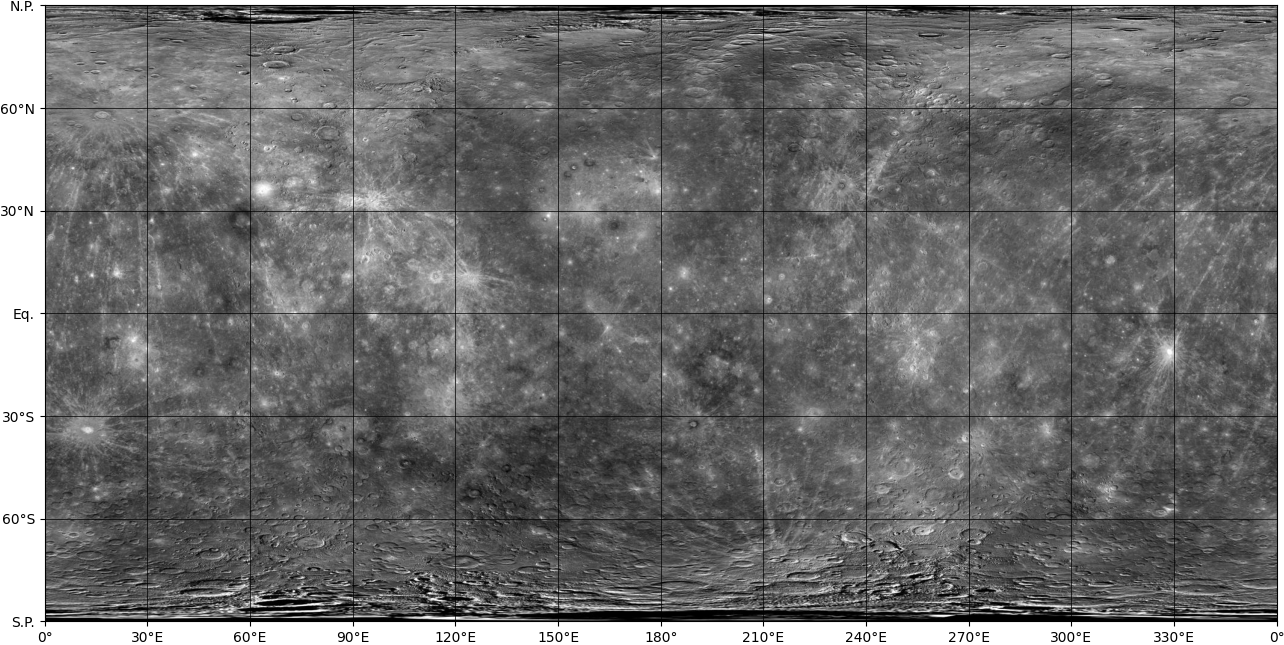
Source: USGS
Original image size: 46,080 × 92,160 pixels
Instrument: Messenger WAC/NAC at 750 nm
Equatorial resolution: 166 m / pixel
Mean radius: 2,439.7 km (from pck00010.tpc kernel).
Venus#
from planetary_coverage import VENUS
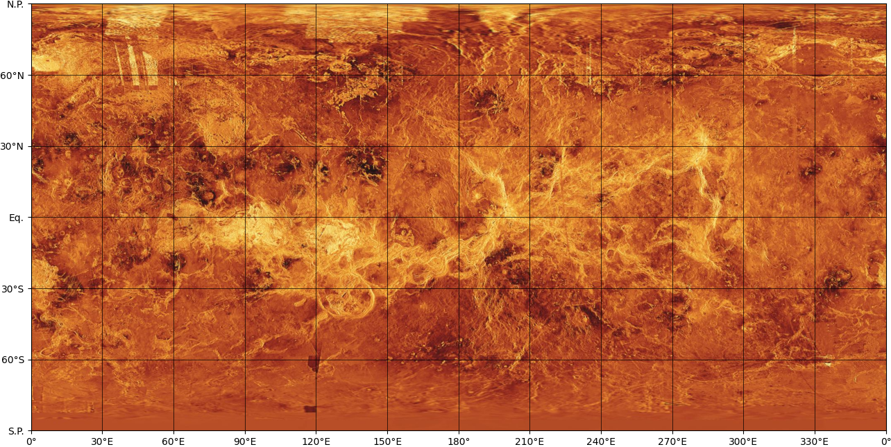
Source: USGS
Original image size: 8,192 × 4,096 pixels
Instrument: C3-MDIR Synthetic Color Mosaic
Equatorial resolution: 4.6 km / pixel
Mean radius: 6,051.8 km (from pck00010.tpc kernel).
Earth#
from planetary_coverage import EARTH
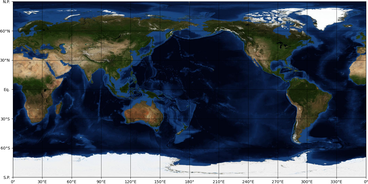
Source: NASA Blue Marble
Original image size: 86,400 × 43,200 pixels
Instrument: Terra MODIS
Equatorial resolution: 463 m / pixel
Mean radius: 6,371.0 km (from pck00010.tpc kernel).
Moon#
from planetary_coverage import MOON
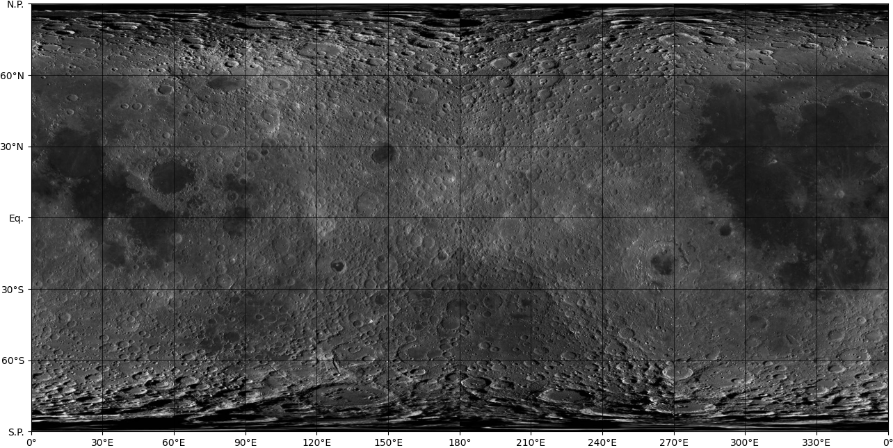
Source: USGS
Original image size: 109,164 × 54,582 pixels
Instrument: LRO WAC
Equatorial resolution: 100 m / pixel
Mean radius: 1,737.4 km (from pck00010.tpc kernel).
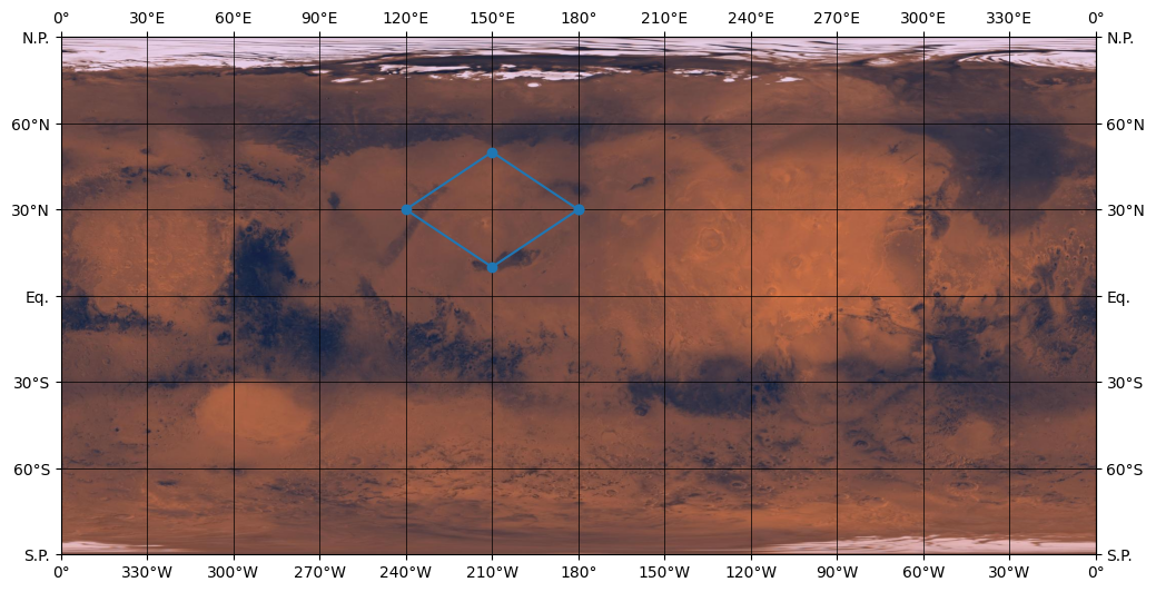
Mars#
from planetary_coverage import MARS
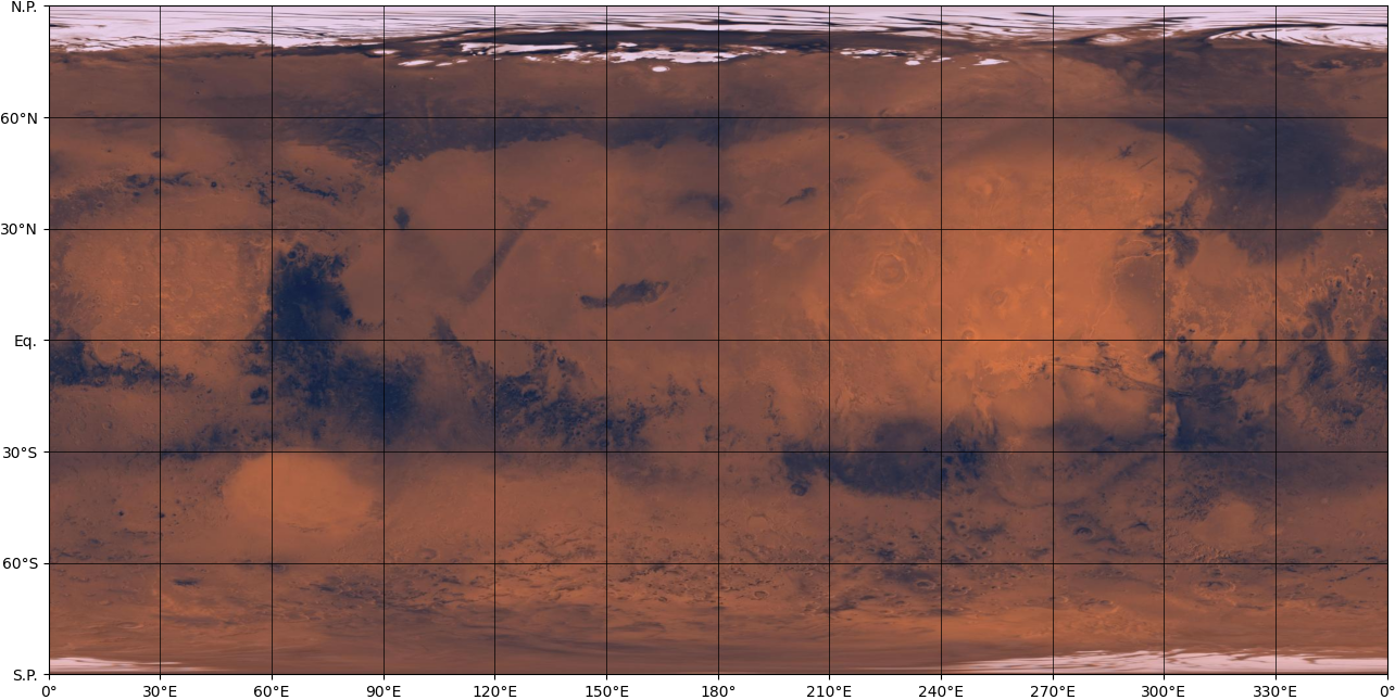
Source: USGS
Original image size: 11,530 × 23,059 pixels
Instrument: Viking Orbiter (red and violet filters)
Equatorial resolution: 925 m / pixel
Mean radius: 3,389.5 km (from pck00010.tpc kernel).
Jupiter#
Warning
For the Giant Planets (Jupiter, Saturn, Uranus and Neptune) the background maps provided here are just for illustrative purposes but don’t really represent the location of the main feature on the top of the atmosphere (since they drift rapidly with time).
This map should be consistent with other planning tools (Cosmographia, MAPPS, Juice Pointing Tool and Gfinder).
from planetary_coverage import JUPITER
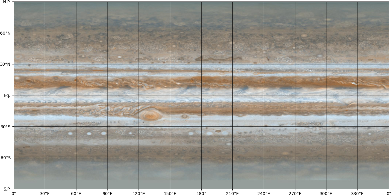
Source: JPL PIA07782
Original image size: 3,601 × 1,801 pixels
Instrument: Cassini ISS
Equatorial resolution: 122 km / pixel
Mean radius: 69,911.3 km (from pck00010.tpc kernel).
Io#
from planetary_coverage import IO
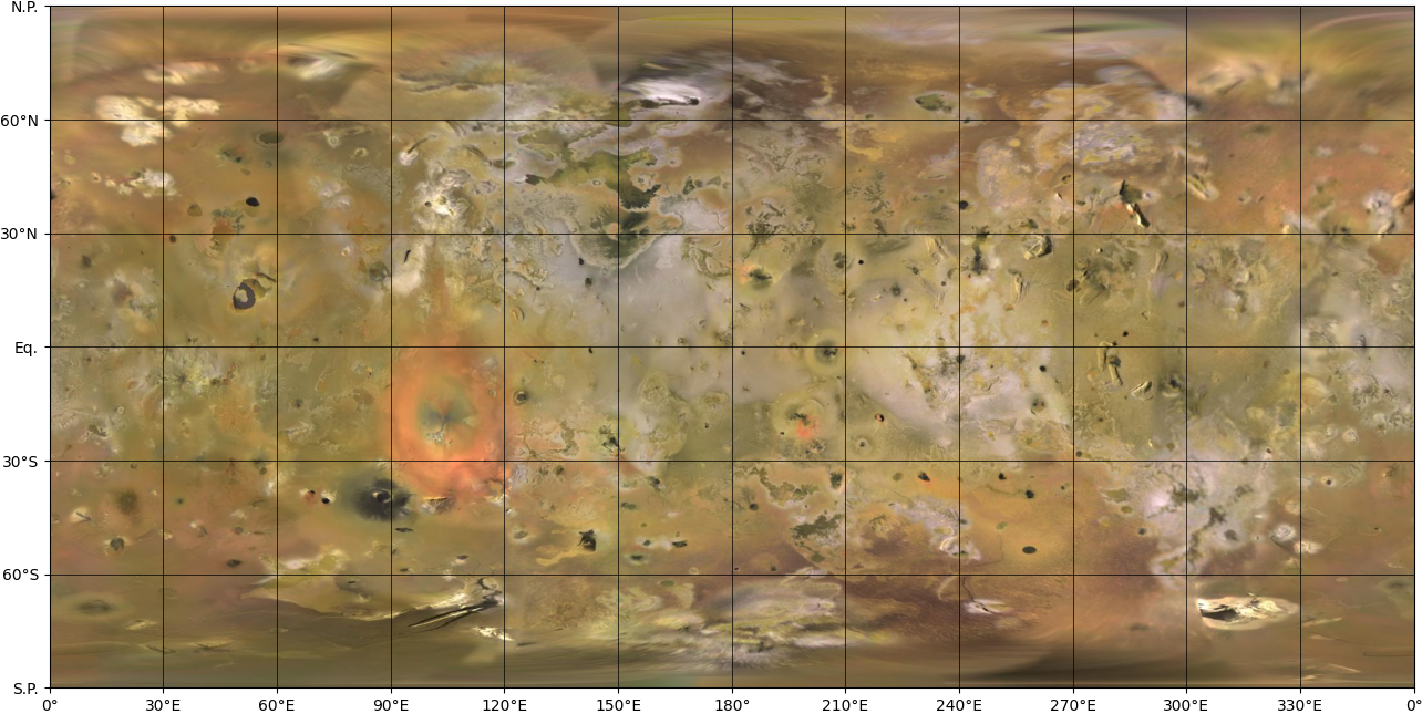
Source: USGS
Original image size: 11,445 × 5,723 pixels
Instrument: Voyager ISS / Galileo SSI
Equatorial resolution: 1 km / pixel
Mean radius: 1,821.5 km (from pck00010.tpc kernel).
Europa#
from planetary_coverage import EUROPA
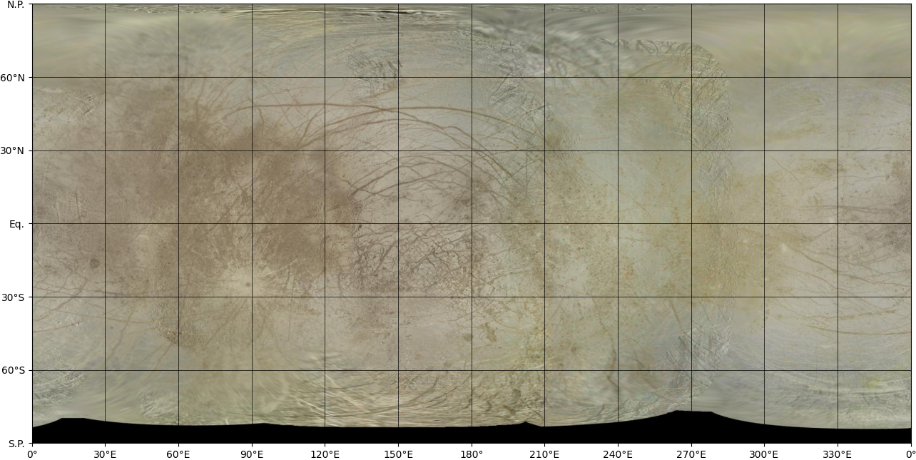
Source: NASA / JPL / Björn Jónsson
Original image size: 20,000 × 10,000 pixels
Instrument: Voyager ISS / Galileo SSI
Equatorial resolution: 490 m / pixel
Mean radius: 1,560.8 km (from pck00010.tpc kernel).
Ganymede#
from planetary_coverage import GANYMEDE
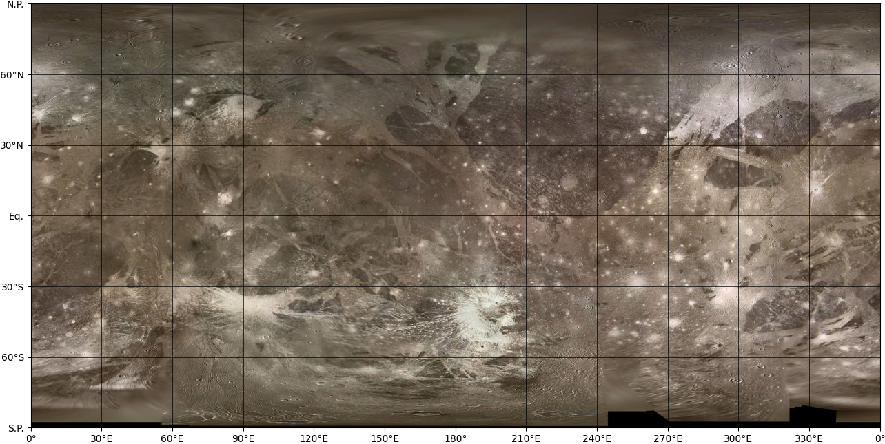
Source: Kersten et al. 2021 - PSS / DLR / Juno colorized with Björn Jónsson map.
Original image size: 46,080 × 23,040 pixels
Instrument: Voyager ISS / Galileo SSI
Equatorial resolution: 360 m / pixel
Mean radius: 2,631.2 km (from
pck00010.tpckernel).
Callisto#
from planetary_coverage import CALLISTO
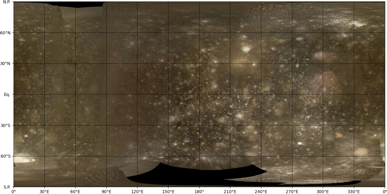
Source: USGS/ESA colorized with Björn Jónsson map.
Original image size: 15,138 × 7,569 pixels
Instrument: Voyager ISS / Galileo SSI
Equatorial resolution: 1 km / pixel
Mean radius: 2,410.3 km (from
pck00010.tpckernel).
Saturn#
from planetary_coverage import SATURN
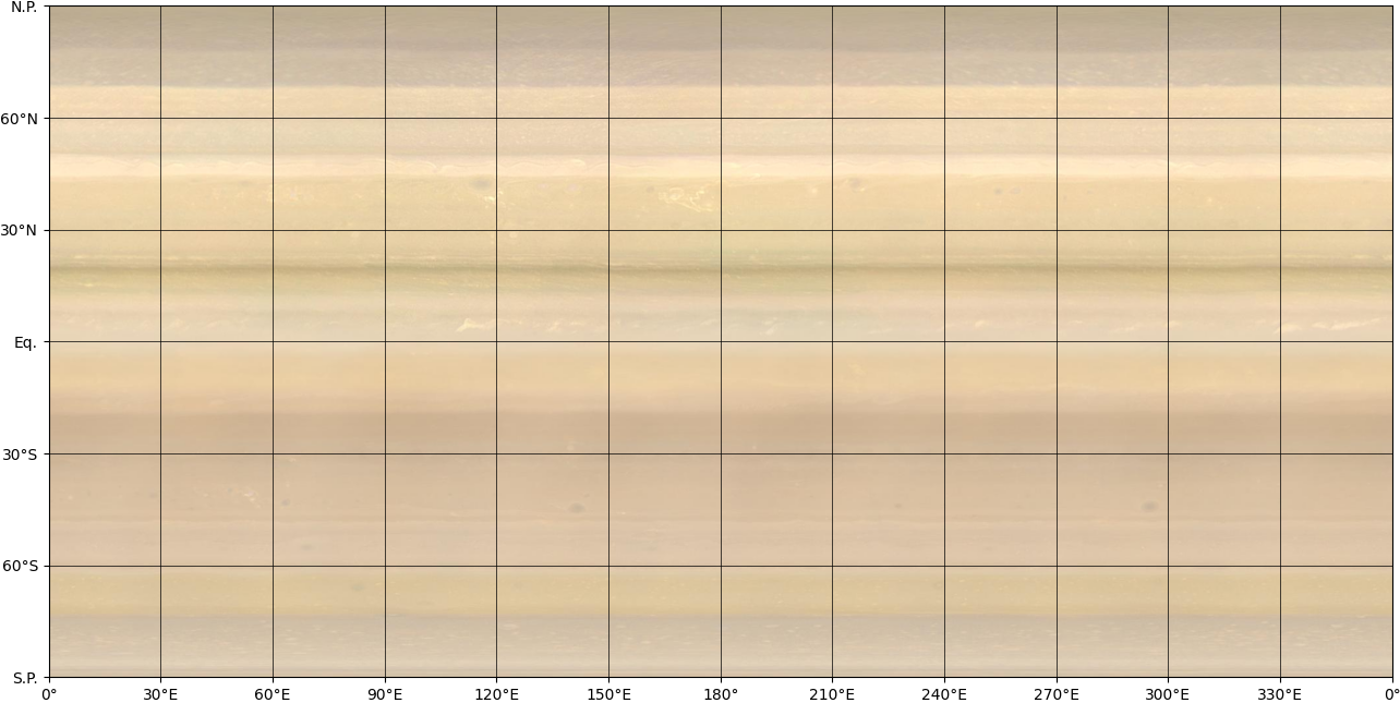
Source: Björn Jónsson
Original image size: 2,880 × 1,440 pixels
Instrument: Cassini ISS
Equatorial resolution: 122 km / pixel
Mean radius: 58,232.0 km (from pck00010.tpc kernel).
Enceladus#
from planetary_coverage import ENCELADUS
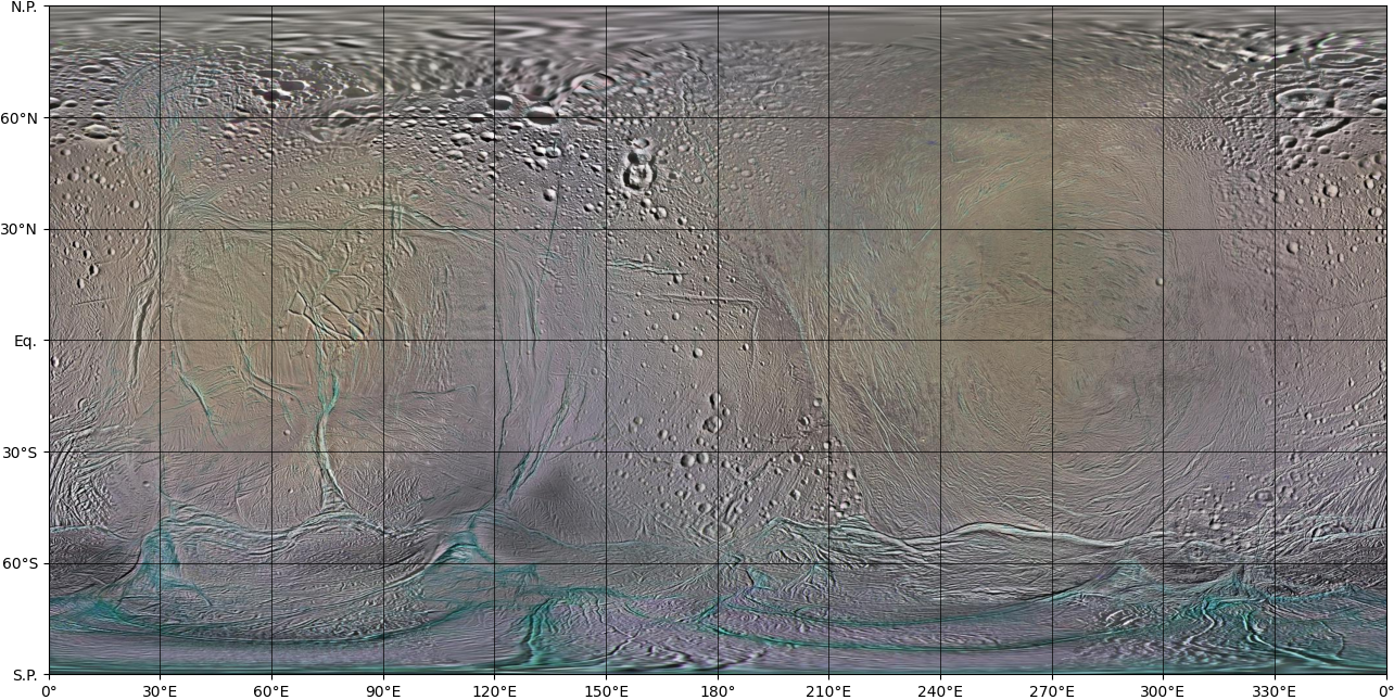
Source: JPL PIA18435
Original image size: 15,960 × 7,980 pixels
Instrument: Cassini ISS (IR3-GRN-UV3)
Equatorial resolution: 100 m / pixel
Mean radius: 252.1 km (from pck00010.tpc kernel).
Titan#
from planetary_coverage import TITAN
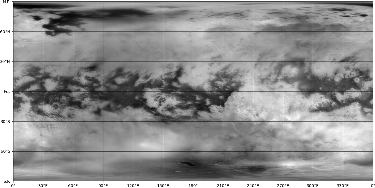
Source: JPL PIA22770
Original image size: 5,760 × 2,880 pixels
Instrument: Cassini ISS (CB3 938 nm)
Equatorial resolution: 2.8 km / pixel
Mean radius: 2,574.8 km (from pck00010.tpc kernel).
Uranus#
from planetary_coverage import URANUS
Original image size: 1 × 1 pixels
Instrument: Voyager ISS
Equatorial resolution: 0 km / pixel
Mean radius: 25,362.2 km (from pck00010.tpc kernel).
Neptune#
from planetary_coverage import NEPTUNE
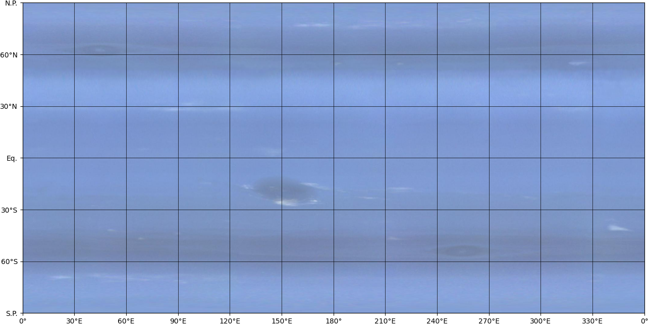
Source: Björn Jónsson
Original image size: 1,800 × 900 pixels
Instrument: Voyager 2 ISS
Equatorial resolution: 86 km / pixel
Mean radius: 24,622.2 km (from pck00010.tpc kernel).
Pluto#
from planetary_coverage import PLUTO
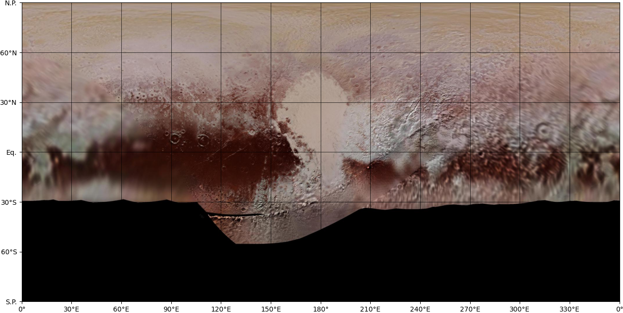
Source: JPL PIA11707
Original image size: 5,926 × 2,963 pixels
Instrument: New Horizon LORRI/Ralph
Equatorial resolution: 1.2 km / pixel
Mean radius: 1,195.0 km (from pck00010.tpc kernel).
Charon#
from planetary_coverage import CHARON
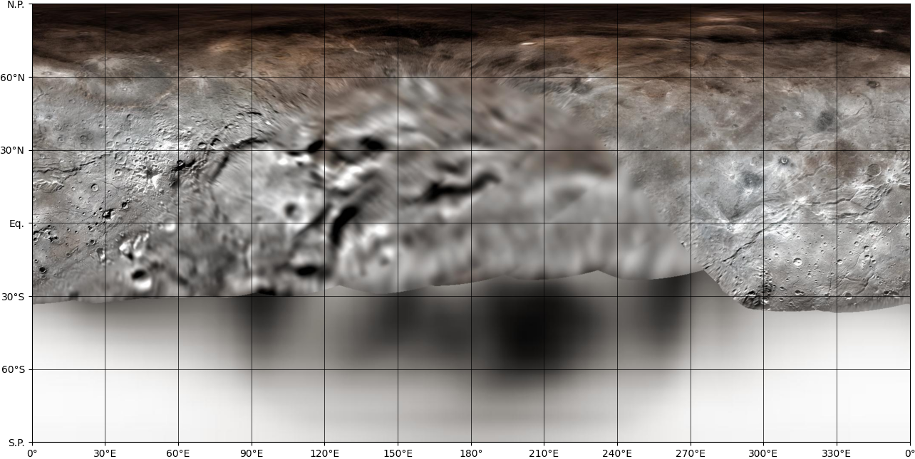
Source: Antdoghalo
Original image size: 12,694 × 6,347 pixels
Instrument: New Horizon LORRI/MVIC
Equatorial resolution: 300 m / pixel
Mean radius: 605.0 km (from pck00010.tpc kernel).
Get a map from the registry#
All the default maps above are also available in the MAPS registry.
This allows you to load a Map programmatically with a string key:
Tip
The target name key is not case sensitive. You can also use a SpiceRef object.
from planetary_coverage import MAPS

MAPS
{'MERCURY': <Map> Mercury | Radius 2439.7 km,
 'VENUS': <Map> Venus | Radius 6051.8 km,
 'EARTH': <Map> Earth | Radius 6371.0 km,
 'MOON': <Map> Moon | Radius 1737.4 km,
 'MARS': <Map> Mars | Radius 3389.5 km,
 'JUPITER': <Map> Jupiter | Radius 69911.3 km,
 'IO': <Map> Io | Radius 1821.5 km,
 'EUROPA': <Map> Europa | Radius 1560.8 km,
 'GANYMEDE': <Map> Ganymede | Radius 2631.2 km,
 'CALLISTO': <Map> Callisto | Radius 2410.3 km,
 'SATURN': <Map> Saturn | Radius 58232.0 km,
 'ENCELADUS': <Map> Enceladus | Radius 252.1 km,
 'TITAN': <Map> Titan | Radius 2574.8 km,
 'URANUS': <Map> Uranus | Radius 25362.2 km,
 'NEPTUNE': <Map> Neptune | Radius 24622.2 km,
 'PLUTO': <Map> Pluto | Radius 1195.0 km,
 'CHARON': <Map> Charon | Radius 605.0 km}
Customize the map#
If none of these maps correspond to your needs, you can create your own custom map by providing a 2:1 background image centered a 180° (preferred) or 0°.
See Map object API for details.
For example, GANYMEDE is defined as:
from planetary_coverage.maps import Map

GANYMEDE = Map('Ganymede_map_180.jpg', body='Ganymede', radius=2631.2)
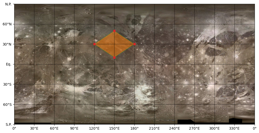
Plot data on the map#
All these planetary maps are expected to be used in matplotlib projection keyword:
lons_e, lats = [180, 150, 120, 150], [30, 50, 30, 10]

polygon = Path([
    (180, 30), (150, 50), (120, 30), (150, 10)
])
fig = plt.figure(figsize=(12, 9))
ax = fig.add_subplot(projection=GANYMEDE)

ax.plot(lons_e, lats, 'o', color='tab:red')

ax.add_path(polygon, facecolor='tab:orange', edgecolor='tab:green', alpha=.5);
Customize the ticks#
You can change the ticks display on the map (east longitude ticks to west longitude ticks, or/and, mirror the ticks on the secondary axis). For example:
Warning
As you see, the input values in ax.plot(lons_e, lats) must be in east longitudes, even if the required ticks representation is 'west'.
fig = plt.figure(figsize=(12, 9))
ax = fig.add_subplot(projection=MARS)

ax.plot([180, 150, 120, 150, 180], [30, 50, 30, 10, 30], 'o-')  # Always east longitude

ax.set_lon_ticks('west')
ax.set_lon_ticks('east', secondary=True)
ax.set_lat_ticks(secondary=True);