Instrument trajectory properties#
List of the available properties#
In this case, its properties are slightly different compared to the SpacecraftTrajectory:
lonlat: the boresight intersection coordinates on the surface (east longitude and latitude).slant: the distance to the surface intersection point from the spacecraft (in km).local_time: the local time computed at the intersection point (in decimal hours).inc: the incidence angle computed at the intersection point (in degrees).emi: the emission angle computed at the intersection point (in degrees).phase: the phase angle computed at the intersection point (in degrees).solar_zenith_angle: the solar zenith angle computed at the intersection point.ra: the right ascension of the boresight pointing in the J2000 frame.dec: the declination of the boresight pointing in the J2000 frame.pixel_scale: cross-track iFOV projected on the target body (km/pixel).fovs: collection of patches of the instrument field of views (see below).
Differences between the InstrumentTrajectory and the SpacecraftTrajectory#
When the orbiter is in a nadir viewing geometry, its trajectory properties correspond (or at least almost equal) to the values retrieved with the SpacecraftTrajectory groundtrack.
However in the general case, the spacecraft can be pointing in any direction and only the points intersecting the surface are considered.
For example:
fig = plt.figure(figsize=(12, 4))
ax = fig.add_subplot()

ax.plot(sc_traj.utc, sc_traj.inc, '--', label='Sub-spacecraft local incidence')
ax.plot(inst_traj.utc, inst_traj.inc, lw=2, label='JANUS instrument boresight local incidence')

ax.legend(loc='lower center', bbox_to_anchor=(.5, 1), ncol=2, frameon=False)

# Optional labels
ax.set_ylabel('Incidence')
ax.xaxis.set_major_formatter(date_ticks)
ax.yaxis.set_major_formatter(deg_ticks);
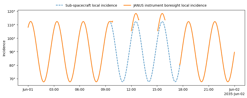
In the above plot, we can see:
the JUICE spacecraft is pointing in the nadir direction (
z-axistowards the targeted body): the orange solid line overlaps with the blue dashes.after ~10h the spacecraft changed its attitude to point in a direction away from the target (towards the Earth for a downlink window): the solid orange line is only present when the
z-axishappens to cross the surface, but, in the general case, this point is different from the sub-spacecraft point (therefore their incidence is different).after ~8h of downlink, the spacecraft is pointing once more in the nadir direction and the 2 lines overlap again.
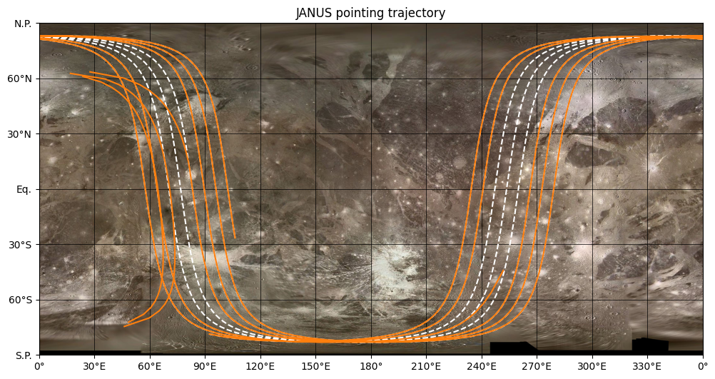
Instrument trajectory on a Map#
We can also see which parts of the orbit are dedicated to the downlink by projecting the data on the map:
fig = plt.figure(figsize=(12, 9))
ax = fig.add_subplot(projection=GANYMEDE)

ax.plot(sc_traj, color='white', ls='--')
ax.plot(inst_traj, color='tab:orange')

ax.set_title('JANUS pointing trajectory');