Spacecraft trajectory properties#
When the temporal window of the Trajectory is selected, you can use it to retrieve many SPICE calculations results directly as properties.
For example, for a SpacecraftTrajectory, the sub-spacecraft point on the surface
(expressed as planetocentric coordinates) can be retrieved with the lonlat property:
sc_traj.lonlat
(array([106.33523534, 106.00961698, 105.69268877, ..., 108.95065025,
         99.57972796,  92.3330836 ]),
 array([-26.50341796, -24.57483397, -22.64463689, ..., -81.24730072,
        -80.05406748, -78.65922961]))
Important
By default, all the SPICE calculations are performed with the approximation abcorr='NONE'.
You can change this behavior at the TourConfig level by providing a abcorr argument with any
valid aberration correction key.
List of the available properties#
Here is a list of the main helpers that are easily accessible to the user on a
SpacecraftTrajectory:
ets: the ephemeris time of the observer.utc: the UTC time of the observer.lonlat: the sub-spacecraft point groundtrack (east longitude and latitude).alt: the altitude of the spacecraft above the the sub-spacecraft point (in km).dist: the distance between the spacecraft and the target body center (in km).target_size: the angular target size seen from the spacecraft (in degrees).local_time: the local time of the sub-spacecraft point (in decimal hours).inc: the incidence angle at the sub-spacecraft point location (in degrees).emi: the emission angle at the sub-spacecraft point location (in degrees).phase: the phase angle at the sub-spacecraft point location (in degrees).solar_zenith_angle: the solar zenith angle (angle between the local normal and the local sub-solar vector).solar_longitude: the seasonal solar longitude (computed on the parent body for the moon, in degrees).true_anomaly: the true anomaly angle from the moon perijove (in degrees)groundtrack_velocity: the groundtrack velocity (speed motion of the sub-spacecraft point, in km/s)ss: the sub-solar point groundtrack (east longitude and latitude).
These properties are stored in numpy arrays and are fully compatible with matplotlib
plot functions. For example:
Note
SPICE computations on the Trajectory properties are performed once and cached to improve performance.
sc_traj.dist
array([3132.67191053, 3131.81832048, 3130.9513112 , ..., 3148.34318997,
       3148.34255504, 3148.30867154])
sc_traj.alt
array([501.47191053, 500.61832048, 499.7513112 , ..., 517.14318997,
       517.14255504, 517.10867154])
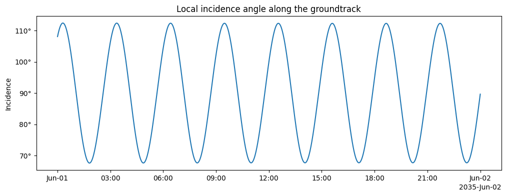
Example of temporal plot#
To represent the evolution of the incidence angle as a function of time, you only need to do:
import matplotlib.pyplot as plt

from planetary_coverage.ticks import date_ticks, deg_ticks, km_ticks
fig = plt.figure(figsize=(12, 4))
ax = fig.add_subplot()

ax.plot(sc_traj.utc, sc_traj.inc)

# Optional labels
ax.set_ylabel('Incidence')
ax.xaxis.set_major_formatter(date_ticks)
ax.yaxis.set_major_formatter(deg_ticks)
ax.set_title('Local incidence angle along the groundtrack');
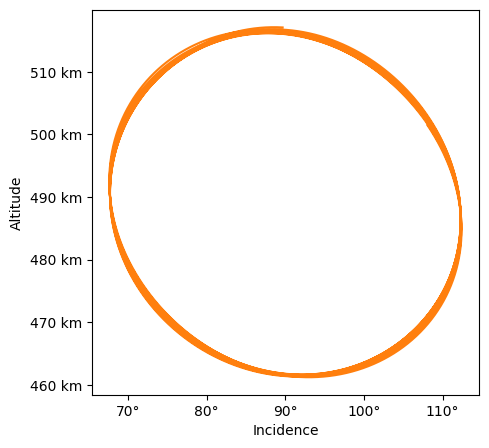
Example of a correlation plot#
You can also correlate different properties:
fig = plt.figure(figsize=(5, 5))
ax = fig.add_subplot()

ax.plot(sc_traj.inc, sc_traj.alt, color='tab:orange')

# Optional labels
ax.set_xlabel('Incidence')
ax.set_ylabel('Altitude')
ax.xaxis.set_major_formatter(deg_ticks)
ax.yaxis.set_major_formatter(km_ticks);
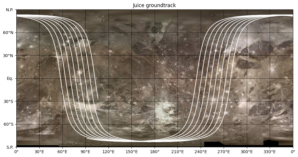
Example of projection on a Map#
The tool comes with a collection of pre-build basemaps that can be use to project trajectory data onto them.
Warning
The selected basemap must have the same name as the trajectory target.
Otherwise an ProjectionMapTargetError will be thrown to avoid
mis-representation of the data.
from planetary_coverage import GANYMEDE
fig = plt.figure(figsize=(12, 9))
ax = fig.add_subplot(projection=GANYMEDE)

ax.plot(sc_traj, color='white', ls='-')

ax.set_title('Juice groundtrack');
More maps are available here.
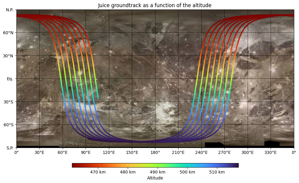
You can also add a 2nd argument (as a string), to color code directly the trajectory with a given property:
fig = plt.figure(figsize=(12, 9))
ax = fig.add_subplot(projection=GANYMEDE)

ax.plot(sc_traj, 'alt', linewidth=3)

ax.set_title('Juice groundtrack as a function of the altitude');