Instrument field of views#
In the example below, we will work on the 2nd flyby of Ganymede (2G2) in February 2032 seen by the JANUS instrument with a time step of 10 secondes around closest approach:
Tip
You can omit the time parts like T00:00:00, :00:00 or :00.
janus_flyby = tour['2032-02-13T22':'2032-02-14':'10 sec'].new_traj(instrument='JANUS')

janus_flyby
<InstrumentTrajectory> Observer: JUICE_JANUS | Target: GANYMEDE
 - UTC start time: 2032-02-13T22:00:00.000
 - UTC stop time: 2032-02-14T00:00:00.000
 - Nb of pts: 721
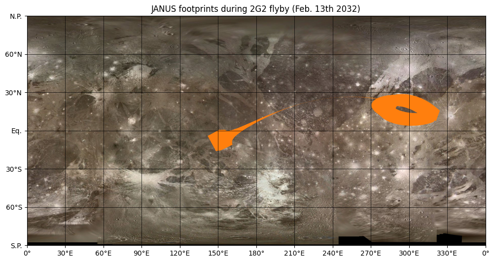
Instrument FOVs on a Map#
By default, the trajectory represented with inst_traj correspond to the surface intersection with the instrument boresight on the target surface. In general, this point is in the middle of the instrument field of view (FOV).
However, instead of representing only the boresight intersection on the surface (like we seen before), it is possible to represent the complete instrument field of view patches on the surface.
To do that, you can use the .fovs property to retrieve a FovsCollection object that can be added on the map:
fig = plt.figure(figsize=(12, 8))
ax = fig.add_subplot(projection=GANYMEDE)

ax.add_collection(janus_flyby.fovs)

ax.set_title('JANUS footprints during 2G2 flyby (Feb. 13th 2032)');
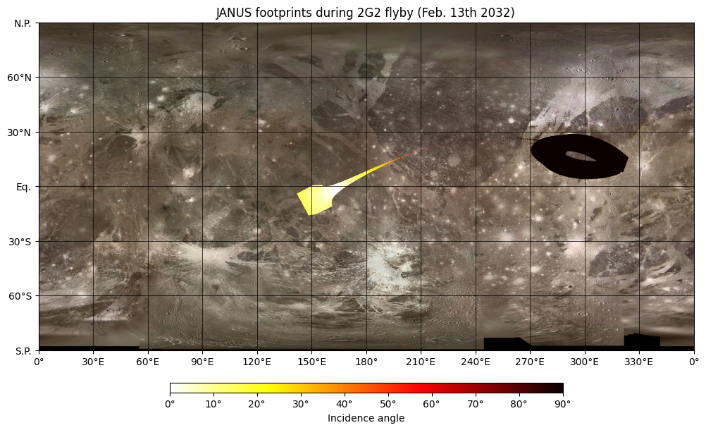
The color of the patches and their contours can be customized by the user with an InstrumentTrajectory property:
Caution
By default, the patches are represented in chronological order and can mask the smaller patches below them. To solve that problem, you can add a sort argument with a given property name to reorder the patches before displaying them.
fig = plt.figure(figsize=(12, 8))
ax = fig.add_subplot(projection=GANYMEDE)

ax.add_collection(janus_flyby.fovs(facecolors='inc',
                                   vmin=0, vmax=90, cmap='hot_r',
                                   sort='inc'))

ax.colorbar(vmin=0, vmax=90, label='inc', cmap='hot_r')

ax.set_title('JANUS footprints during 2G2 flyby (Feb. 13th 2032)');
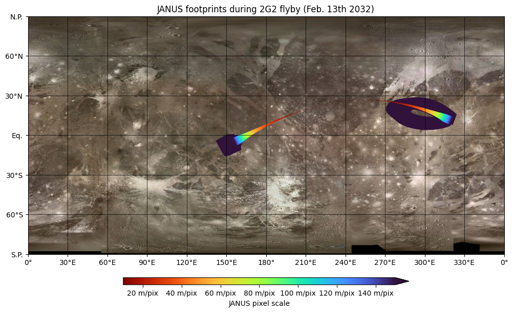
Customize the colorbar#
You can customize the colorbar and change its label and ticks.
For example, let say that you want to display JANUS pixel scale, not in km/pix but in m/pixel, you can import a custom formatting ticks (m_pix_ticks) and provide it to the format attribute.
Tip
You can add a reverse boolean argument to change how the patches are sorted (ascending or descending values). By default, the sort goes from the small values first (below) to the large values (on top), except for inc, dist and alt that are expected to be reversed.
from planetary_coverage.ticks import m_pix_ticks

fig = plt.figure(figsize=(12, 8))
ax = fig.add_subplot(projection=GANYMEDE)

ax.add_collection(janus_flyby.fovs(facecolors='pixel_scale',
                                   vmin=0.01, vmax=.15,
                                   sort='dist', reverse=True))

ax.colorbar(vmin=0.01, vmax=0.15, label='JANUS pixel scale',
            format=m_pix_ticks, extend='max')

ax.set_title('JANUS footprints during 2G2 flyby (Feb. 13th 2032)');
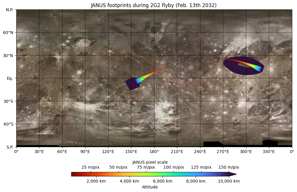
Caution
In a previous release, we introduce an ax.twin_colorbar() helper to represent dual values (altitude vs. pixel scale).
This method, shown below, still works and can be used to get a rough estimate of the instrument pixel resolution
for a SpacecraftTrajectory in nadir looking geometry. You must keep in mind that pixel_scale
in InstrumentTrajectory objects provide an better representation of the pixel scale projected on the surface
where the instrument boresight actually intersect the surface. We highly recommend to use the method above,
rather than the method below to represent the instrument pixel scale.
fig = plt.figure(figsize=(12, 8))
ax = fig.add_subplot(projection=GANYMEDE)

ax.add_collection(janus_flyby.fovs(facecolors='alt',
                                   vmin=500, vmax=10_000,
                                   sort='dist', reverse=True))

ax.colorbar(vmin=500, vmax=10_000, label='alt', extend='max')
ax.twin_colorbar(label='JANUS pixel scale',
                 ticks=[25, 50, 75, 100, 125, 150],
                 format=janus_flyby.observer.ifov_cross_track * m_pix_ticks)

ax.set_title('JANUS footprints during 2G2 flyby (Feb. 13th 2032)');